Environmental exposure - higher tier approaches

Background
Standard assessments are calculations based on conservative, generalising assumptions and simple equations. Calculations can be e.g. performed using Microsoft Excel spreadsheets, sometimes provided as standardised 'tool' by the respective authorities, or slightly more sophisticated models (e.g. the FOCUS suite for EU groundwater and surface water modelling) but still using conservative input parameters. In contrast, higher tier approaches gradually increase in complexity with each modelling tier in order to depict the natural "real-life" conditions and possible effects as accurately as possible. In the following, we explain how higher tier approaches can be used in assessments to demonstrate the safe use of a product - using an example from crop protection.
Modern agriculture often relies on the use of pesticides in order to maintain a high production level. However, a fraction of the pesticide applied to agricultural fields can reach surface waters and groundwater via a number of different pathways and can cause harmful effects to the environment. Computer simulations are being frequently applied in the authorisation process of pesticides in order to evaluate the risk for the environment or in the frame of water stewardship projects and are usually performed in a tiered approach.
Amongst the various higher tier approaches (e.g. spatial groundwater modelling, vulnerability mapping, effect modelling), catchment modelling is a higher tier option for ecological risk assessment as stated in the FOCUS Landscape & Mitigation guidance (2002). The EFSA Guidance Document on Aquatic Risk Assessment (EFSA, 2013) indicates a key role for effect modelling in future aquatic risk characterization in a tiered risk assessment framework. Such approaches require correspondingly adapted exposure tools and scenarios ranging from simple edge-of-field to spatio-temporally explicit landscape-scale catchment models. These approaches should be sufficiently flexible and transparent in order to design lower- and higher-tiers of consistent protection levels.
knoell experts have been working in a variety of projects focussing on the different facets of higher-tier approaches for years, an overview of their work can be found in knoell's publication section (e.g. He et al., 2017, Reichenberger et al., 2018) and a more detailed example is given below (also Multsch et al., 2018, Multsch et al., 2019).
The regulatory catchment model
The regulatory catchment model is a new model currently in development by Bayer AGa, knoell Germany GmbHb and University Giessenc. It is a modular, flexible and scalable (in time and space) toolbox in order to provide solutions for future regulatory requirements and refinement options in aquatic risk assessment of plant protection products. The toolbox allows for stepwise adaption of model complexity to address tiered risk assessments. The approach is based on the open-source hydrological programming library CMF (Kraft et al., 2011) . The unique advantages of the newly developed approach are as follows:
Adapting the hydrological model structure within a consistent geospatial catchment discretisation. The user has then the oppertunity to select from three different options for running the whole catchment and one option to simulate only single cells. This is an unique feature of the model, because it provides flexibility in terms of hydrological detail and spatial representation of the catchment.
Integrating 1d models into fully connected catchment scale flow regimes. The model allows for the utilisation of timeseries from established 1d models of FOCUS risk assessment, e.g. MACRO or PRZM, and to connect them in a spatial manner in order to simulate water and solute transport across entire catchments.
Grouping single areas in catchments on the basis of unique combinations of natural properties. In larger catchments environmental data is often similar for single fields (e.g. climate x soil x management). Such fields can be summarized as unique combinations, which can be simulated one time by using the ‘1dField’ option and afterwards related to localised cells using within the ‘timeseriesCatchment’ option. This approach can save a lot of simulation time, because the complexity of individual setups is reduced, but the spatial discretisation stays in place.
Handling data efficiently and transparently. The user can select between the two formats CSV and HDF5. CSV gives the user easy access to modelling data by using a text editor or MS Excel, which is a good choice for small scale / short term analysis. When simulating larger areas for long time periods disk space and data transfer time could be a limiting factor. HDF provides the ability to create compressed binary files, which reduce the required disk space in a high extent and can be accessed and processed by specific libraries of scripting programming languages such as R (h5) or Python (h5py).
The model is implemented following an object-oriented programming approach using Python3. Natural entities and their relation to each other are defined by a has-a-relationship. The numerical calculations are done by the CMF library which is implemented in C++ and makes use of the CVODE solver. Model documentation is done by using sphinx and model versions are managed by TortoiseSVN. When programming the model a focus was on using well established open-source Python packages with a widespread use by science, authorities and industry as well as by other third party software in the field of geoanalysis (e.g. ESRI ArcPy):
- Multi-dimensional array processing with numpy,
- Statistics with scipy and pandas,
- spatial oeprations with scipy.spatial and shapely as well as
- plotting with matplotlib.
The following paragraphs give a brief overview of the model.
Example
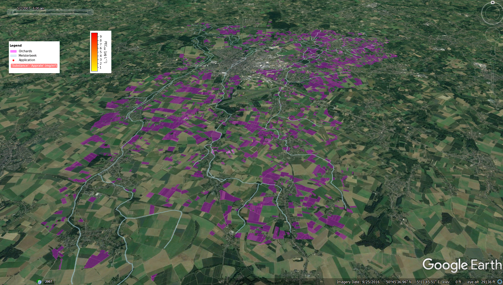
Drift from agricultural fields to aquatic systems related to plant protection product application is a major issue to be addressed in aquatic risk assessment. Using the newly developed catchment model the regulatory relevant concentrations in sediment and water can be assessed. The spatial (i.e. size and number of single river segments) and temporal resolution (hourly) are set by the user to match the relevant scale for a consecutive aquatic ecotoxicolocial risk assessment.
The example shows a large scale catchment (ca. 1600 river segments which sum up to 150 km) in Belgium with a dense river network and an intensive cultivation of pome fruits (purple areas). The case study shows the predicted environmental concentration in surface water (PECsw) after an application of a fungicide to all pome fields at the beginning of May. The video covers a period of eight days after the application.

Modelling concept
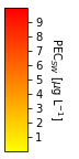
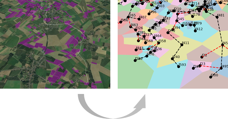
The catchment with all its components, i.e. forests, fields, rivers and urban areas, is divided into a set of cells and river segments which are represented by a set of natural properties and biophysical processes. The information on the spatial location, extent and land use must be obtained from land use cover data from publicly available resources (e.g. CORINE Land Cover , European catchments and Rivers network system) or local authorities.
The modelling process starts with an automated connection of cells and river segments. Optionally, the catchment can be discretised in smaller units. The user has then the opportunity to select from three different options for running the whole catchment and one option to simulate only single cells. This is an unique feature of the model, because it provides flexibility in terms of hydrological detail and spatial representation of the catchment.
Options (a)-(c) provide the same output for each river segment in the catchment, but differ in the calculation method of water flow across land areas:
(a) completeCatchment: The entire flow network of the catchment is simulated including river segments and cells. All fluxes are simulated by CMF on the basis of climate and soil data.
(b) timeseriesCatchment: The entire flow network of the catchment is simulated including river segments and cells. The fluxes from single cells must be provided as time series for surface runoff, drainage flow and groundwater flow. Theses flows can be calculated using the '*1dField' option or by any other 1D field scale model such as MACRO or PEARL.
(c) areayieldCatchment: Only the stream network is simulated. In order to simulate the inflow into each reach, the area weighted inflow is calculated by multiplying the related catchment area by observed flow. The catchment area is calculated on the basis of the cumulative areas of cells which are connected directly or indirectly to the reach.
The final option differs from the previous ones:
(d) 1dField: Only single fields are simulated with a 1D simulation approach. The soil is divided into several layers, as well as holds a surface, drainage and groundwater flow. This approach is equal to the field representation of 'completeCatchment', but without connecting the cells across the catchment.
Why use different options? In larger catchments environmental data is often similar for single fields (e.g. climate x soil x management). Such fields can be summarized as unique combinations which can be simulated one time (using ‘1dField’ option) and afterwards related to localised cells using the ‘timeserisCatchment’ option. This approach can save a lot of simulation time, because the complexity of individual setups is reduced, but the spatial discretisation stays in place. Moreover, the 'timeseriesCatchment' option allows the utilisation of time series from established 1d models of FOCUS risk assessment, e.g. MACRO or PRZM.
Quick user guide
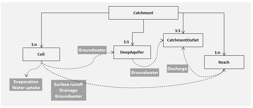
Data structure
The data structure consists of three hierarchical levels. The ‘runlist’ holds a list with all ‘projects’ as a well as information regarding simulations period, number of threads and the hydrolocial modellign option. Projects are grouped in single folders. Each folder represents a model run which can be a single agricultural field, a network of river segments or an entire fully distributed catchment. The folder contains all input data files, e.g. climate and soil information, crop management and a list of cells, reaches and other spatial units of the catchment.
Pre-processing
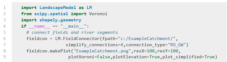
A set of pre-processing tools is available, e.g. to create a flow network between single cells and river segments. The algorithm calculates Thiessen-Polygons between all cells in the first step. Adjacent cells are connected to each other via surface water, drainage and groundwater flow. An iterative adaption procedure simplifies the number of connections in order to reduce the complexity of the flow network.
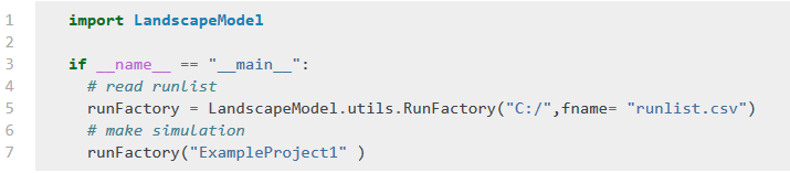
Simulation
The model can be executed by using a Python script and calling the related functions:
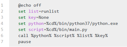
… or by using a batchfile which will execute all simulations as defined in the ‘runlist’:
Post-processing
Various functions are available to prepare graphs and summaries of the simulation:
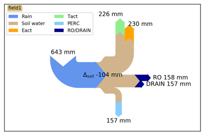
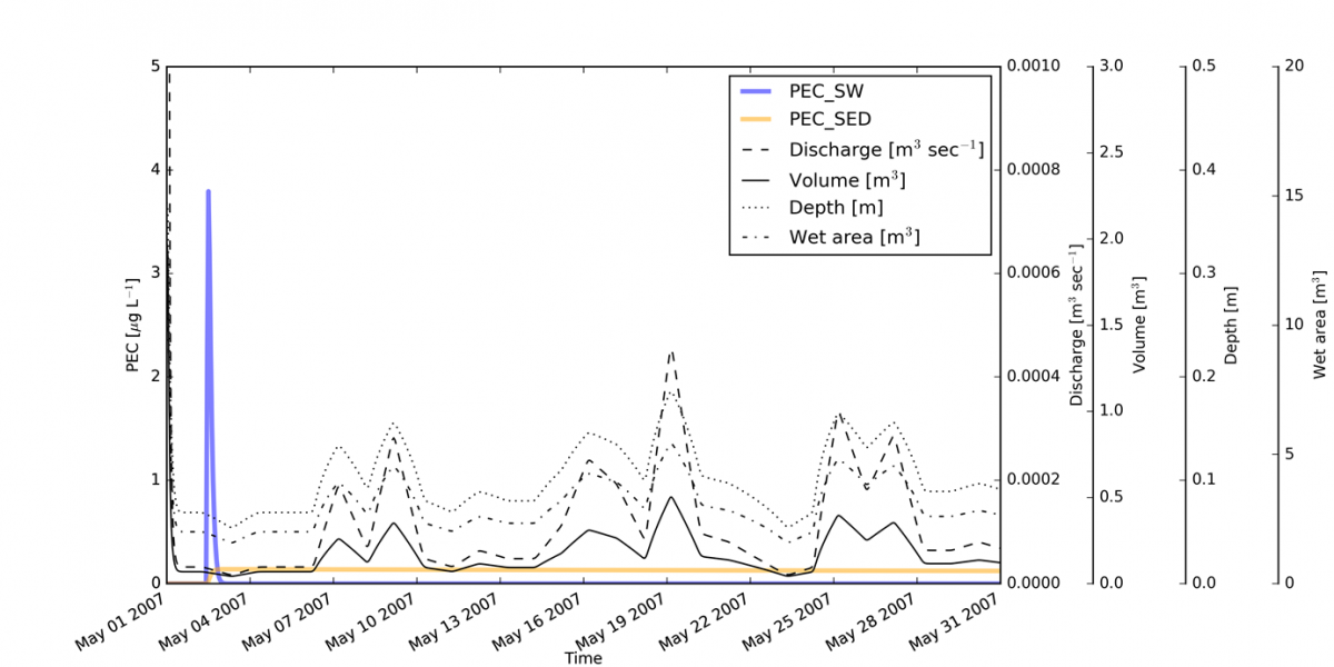
The water and solute balance of single river segments can be evaluated in detail:
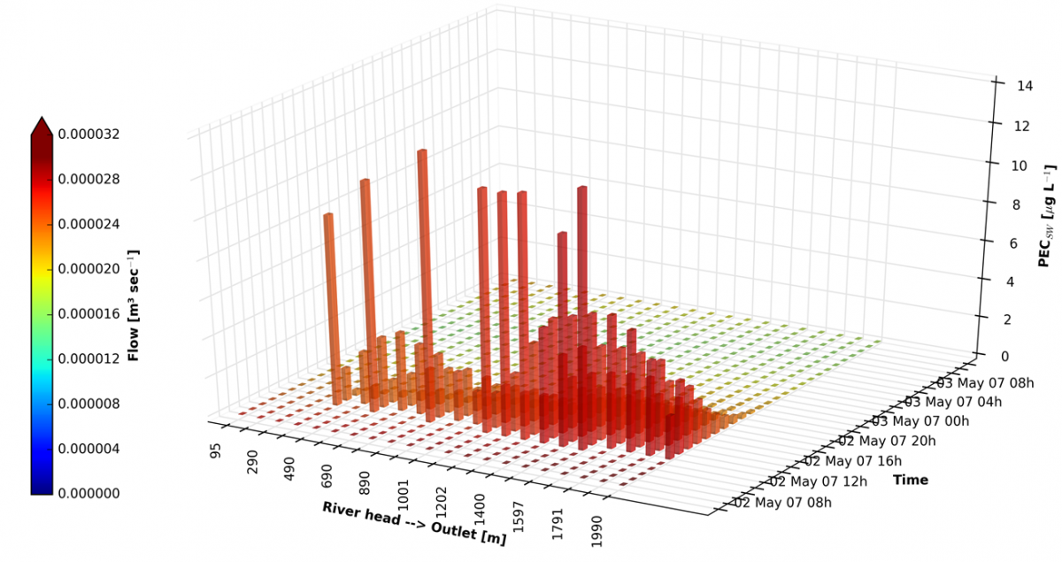
PEC values of several consecutive river segments can be evaluated over space and time:
a Thorsten Schad; b Sebastian Multsch, Florian Krebs, Stefan Reichenberger; c Philipp Kraft, Lutz Breuer